repository

what am I looking at?

I made some raytraced images of a wormhole following this paper by James, von Tunzelmann, Franklin and Thorne using Julia and its illustrious differential equations suite. The wormhole connects two disjoint, asymptotically flat spacetime regions. What a traveller would see traversing the wormhole can be seen in this video.

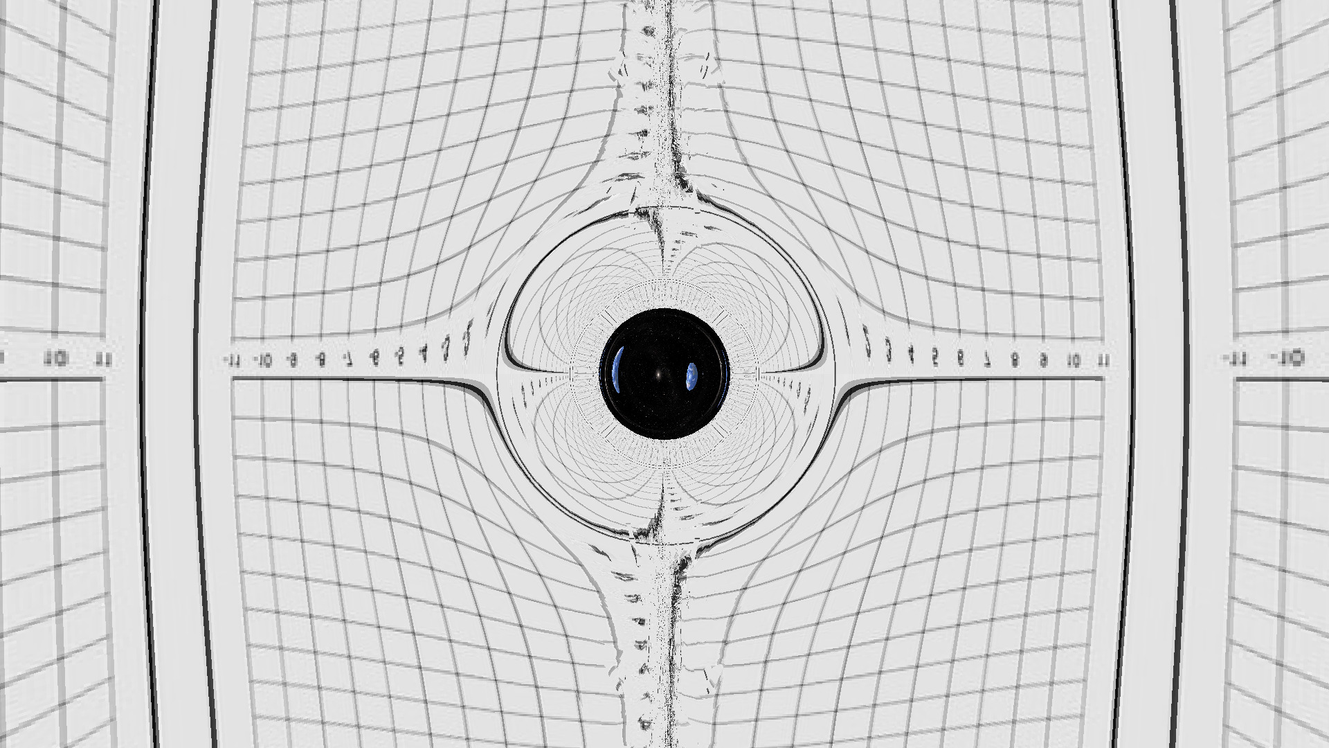
Here are some noteworthy features of the rendering:

• The wormhole itself is spherically symmetric.

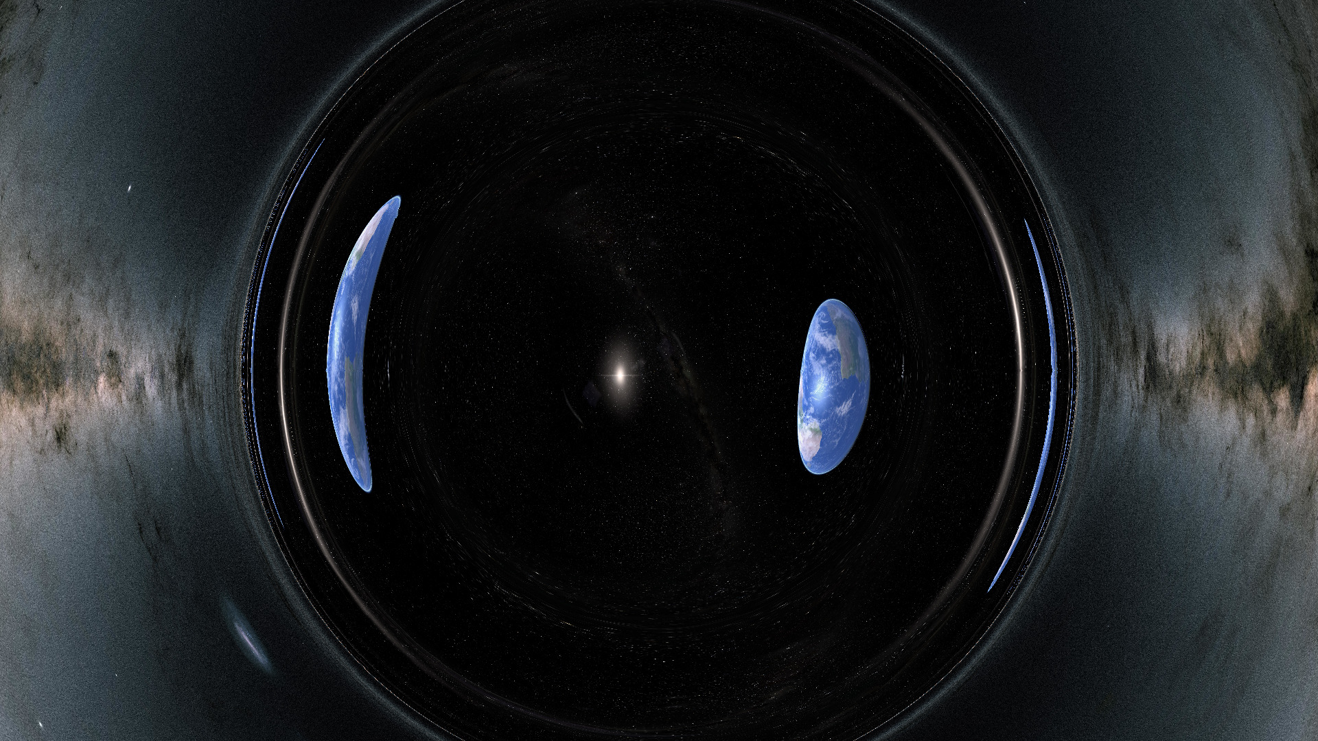
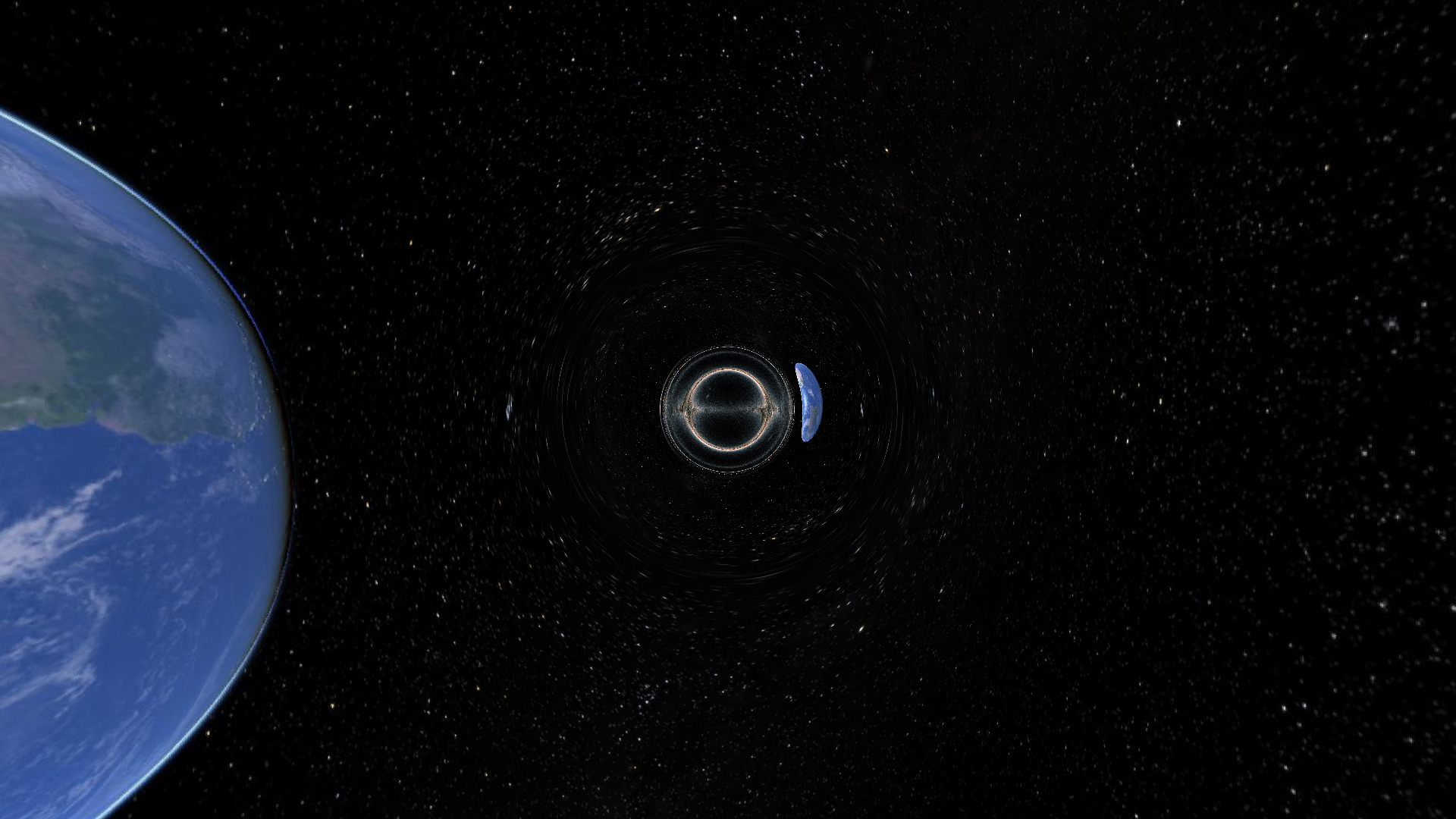
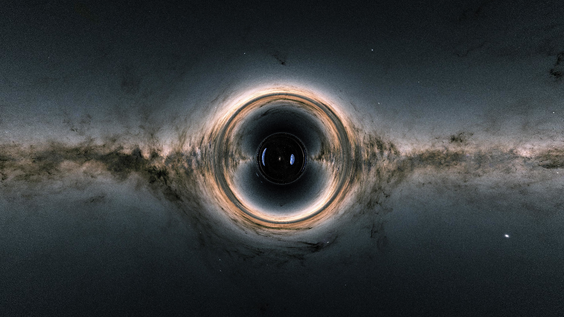
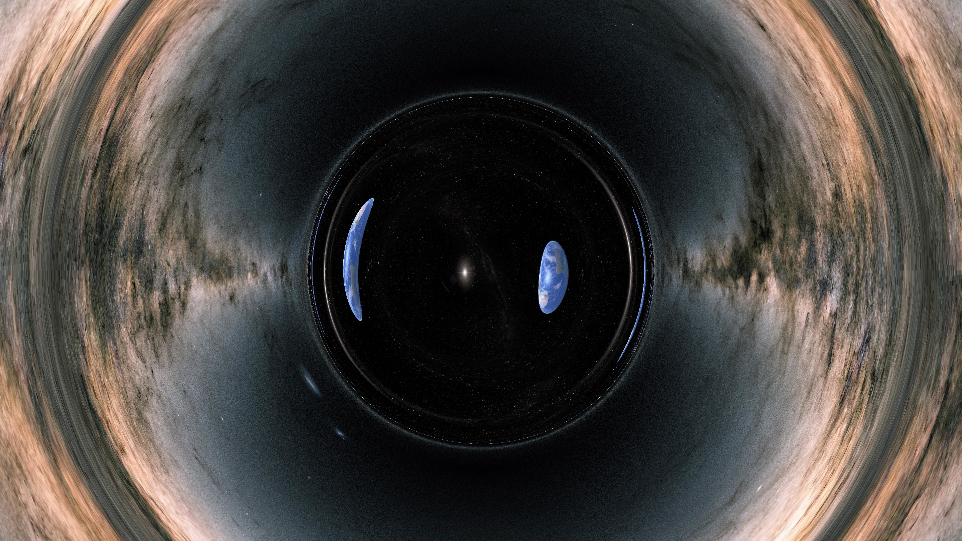
• Light passing near the wormhole is affected by gravitational lensing. This is qualitatively similar to the gravitational lensing from other compact, massive bodies such as black holes and neutron stars. In the above video, the image of Earth on the right comes from light passing along the opposite side which has been redirected toward the camera.

• Light passing through the wormhole gets stuck and can wrap around its circumference multiple times. This is most easily seen in the multiple "squashed" images of Earth on the interior of the wormhole in the image at the top of the page. A way to picture this is to think of the rays of light passing through the wormhole like the stripes on a candy cane. The direct rays form the least distorted image, while rays at other angles wrap around to form the distorted images.

The existence of a traversable wormhole in the real universe would require regions of large negative energy density, and even then are thought to suffer from blueshift instabilities. This rendering is physically realistic in that it accurately depicts the effect of such a large negative energy density on light according to pure Einstein gravity, but unrealistic in that such a large negative energy density either can't exist or is badly unstable. The effects of the gravitational lensing outside of the wormhole, however, are similar to that of real objects. For example, a black hole without any bright crap falling into it would look approximately like the above pictures, with the view through the wormhole replaced by blackness.

Similar raytraced renders using this wormhole metric were used in the abysmal Hollywood movie Interstellar. Unfortunately, the movie's creators did not deem the renderings in the original paper tantalizing enough to inspire a plot any less idiotic than Matthew McConaughey falling into the wormhole and talking to his estranged daughter or some other such contrived and melodramatic nonsense. Fortunately the graphics artists were more talented and provided us with some nice imagery. If you are unfamiliar, I recommend searching for some short clips and images online and save yourself from the experience of watching the film.

raytracing

Raytracing is arguably the most obvious method for rendering images: for each pixel in your image, compute the frequency and intensity of all radiation incident to the corresponding pixel on the imager. While simple in principle this method can easily become computationally intractible. You may have heard that NVidia GPU's, in particular the "RTX" GPU's, can perform raytracing in real time. While impressive, the actual performance isn't quite adequate for gaming in practice without elaborate post-processing prepared from supervised learning.

In NVidia's case, raytracing amounts to solving null geodesics in Minkowski space, or, in other words, drawing straight lines (at least through a medium with a constant index of refraction). Since solutions are not only analytically available at every point but also about as simple as possible to compute it might seem this is not a particularly onerous task, but there are several things to consider which make, say rendering Quake II with pure raytracing quite daunting:

• While the path of the light itself may be trivially simple to compute, the point at which it intersects some geometry may not be.

• There can be all manner of optical aberration both in the scene and inherent to the camera itself, many of which would require more than a single raytracing solution for each pixel.

• Once you determine the point of origin of the light you have to perform the same raytracing process again to determine what it looks like (i.e. what light has arrived at that surface). In principle, this goes on ad infinitum.

I assume that NVidia's raytracing either makes some clever approximations at each of those steps or just skips them entirely. In my case, I can skip almost all of it

• There is nothing on the manifold for the light rays to intersect (whatever imaginary stuff is stabilizing the wormhole is invisible). Every single ray goes all the way out to the infinities on either side of the wormhole where I place static images.

• I model an ideal pinhole camera.

• I just use the two images at either infinity and that's it.

In my case the null geodesics were not analytically solvable and not nearly as simple as straight lines through Euclidean space, so nearly all of the computational effort was spent tracing the rays through empty space.

images at infinity

When I started this project, I was a bit unsure how to find a digital spherical image. It's pretty easy to invent some spherical projections, and wikipedia has a list of many such projections (though it is curiously anthrocentric in calling them "map projections", by which it means a map of Earth), but that doesn't exactly help me find images.

It turns out that what I was looking for is called an equirectangular projection which is pretty much the simplest projection possible if you are using spherical coordinates: the vertical axis is a linear function of the polar angle $\theta$ (with the poles at the edges) and the horizontal axis is a linear function of the azimuth $\phi$, that's it.

Here we have what it looks like inside a cubical room with a grid on each wall if we project it onto a rectangle.

For my infinities I used some nice images from the Gaia telescope.

the wormhole

The paper describes a simple (if rather contrived) spherically symmetric wormhole. There are a number of analytic wormhole solutions in general relativity with spherical or axial symmetry. The most well-known of these is the Schwarzchild solution, but the regions connected through the event horizon in Schwarzchild are causally disconnected. To be able to see (or travel) from one side of the wormhole to another, we need a wormhole metric that connects two regions with timelike geodesics.

There have been a number of wormhole metrics around, but in the paper the authors construct their own. The reason the give is that they want the metric to have multiple free parameters which can be adjusted to obtain a result that "looks cool" (my description, not theirs). The authors call their wormhole the "Dneg" wormhole.

The basic idea of how to write a (spherically symmetric) wormhole is to let the radial coordinate $\ell$ (we will not call it $r$ for reasons which will soon become apparent) go negative.

Now, of course you can just start with Minkowski space written in spherical coordinates

$$ds^{2} = -dt^{2} + d\ell^{2} + \ell^{2}(d\theta^{2} + \sin^{2}(\theta)d\phi^{2})$$

and declare that $\ell\in(-\infty,\infty)$, but this won't do you any good since now you just have two completely disjoint Minkowskian manifolds.

The idea behind creating a wormhole metric is to keep the angular part of the metric $d\theta^{2} + \sin^{2}(\theta)d\phi^{2}$ from ever vanishing. Anywhere this part of the metric doesn't vanish descibes an entire 2-sphere rather than just the point that lies at the center of the spherical coordinate system. To this end, we write

$$ds^{2} = -dt^{2} + d\ell^{2} + r^{2}(\ell)(d\theta^{2}+\sin^{2}(\theta)d\phi^{2})$$

where $r(\ell)$ is some arbitrary function which never vanishes for any $\ell$. In this way, we are passing through spheres for every $\ell$, and we are able to "go past" the $\ell=0$ coordinate singularity of Minkowski space to some other (causally connected) region.

The "classic" wormhole is the Ellis wormhole, which chooses

$$r(\ell) = \sqrt{\rho^{2} + \ell^{2}}$$

for some free parameter $\rho$, which is the starting point of the Thorne paper.

As I had previously mentioned, the paper's authors wanted a wormhole with multiple adjustable parameters. The exact form they chose for $r(\ell)$ isn't that important (if you're curious, read the paper), but it is important to note that their function had the 3 parameters

• $a$ is the "length" of the wormhole. Specifically, they chose $r(\ell)$ to be constant for $-a \le \ell \le a$.

• $\rho$ is the "width" of the wormhole, in particular $r(-a\le \ell\le a)=\rho$.

• $\mathcal{M}$ is the "mass" of the wormhole which governs gravitational lensing caused by the wormhle and the gradualness of the transition from the wormhole to asymptotically flat spacetime.

Like the original authors, when making my renderings, I simply chose arbitrary values for these parmaters which result in cool pictures. Said cool pictures mostly occur when all three parameters are roughly the same order of magnitude.

For fun, I made some additional images showing how the appearance of the wormhole changes with these parameters. As the wormhole is invariant up to an overall rescaling of the 3 parameters, I kept $\rho$ fixed (I also kept the position of the camera fixed, which, in retrospect, can be a bit deceptive).

null geodesics

The one thing that is significantly more complicated in our case than in the most common applications of ray-tracing is that it is non-trivial to compute the null geodesics (paths of a ray of light) and an analytic solution is not readily available. Instead, we must integrate the geodesic equation and we have to do it a lot

I was able to take advantage of some particularly nice tools here, both theoretically and computationally, so I'd like to describe those in a little more detail.

geodesic Hamiltonian

In the Thorne paper, they mention that they compute the geodesics by solving a set of Hamiltonian equations. This is noteworthy because the Hamiltonian formulation in general relativity can make our lives particularly easy. Since they don't talk much about this in the Thorne paper and the technique is curiously absent from most GR textbooks, I will derive it here.

You may have heard that inertial objects travel along paths of minimal proper length. In flat Minkowski space these are just straight lines. In our wormhole metric they are also straight lines (if we define straight line to mean geodesic) but they become non-trivial to compute.

Since the proper length of the trajectory $\gamma$ is given by

$$\int_{\gamma}ds = \int_{\gamma}d\lambda\sqrt{g_{\mu\nu}\dot{x}^{\mu}\dot{x}^{\nu}}$$

where $\lambda$ parameterizes the trajectory and $\dot{x}^{\mu}=dx^{\mu}/d\lambda$. We can simplify things by choosing a Lagrangian which is minimized at the same trajectory but is easier to work with

$$L = \frac{1}{2}g_{\mu\nu}\dot{x}^{\mu}\dot{x}^{\nu}$$

(though note that this involves sacrificing some ability to re-parameterize the trajectory).

This was all well and good, but the Euler-Lagrange equations arising from this $L$ don't really give us that much of a simplification. What does give us a substantial simplification are the Hamiltonian equations. To compute them, recall the Hamiltonian is related to the Lagrangian by the Legendre transformation

$$H = p_{\mu}x^{\mu} - L$$

where $p_{\mu}$ is the canonical momentum defined by $\partial L/\partial \dot{x}^{\mu}$, which in our case is easily computed to be simply $\dot{x}^{\mu}$ (this also reveals why we chose the coefficient of $1/2$ in front of the Lagrangian). The 4-velocity $\dot{x}^{\mu}$ is proportional to the momentum $p^{\mu}$, so I will go on writing the canonical momentum as $p_{\mu}$ since it is the same as the covariant form of the momentum we are all familiar with.

Anyway, we can now see that the Hamiltonian is simply

$$H = \frac{1}{2}g^{\mu\nu}p_{\mu}p_{\nu}$$

It is significant that we chose to write $H$ in terms of the covariant momentum $p_{\mu}$ rather than $p^{\mu}$ because, as we have seen above, it is $p_{\mu}$ and not $p^{\mu}$ which is the canonical momentum, and we therefore must differentiate by $p_{\mu}$ and not $p^{\mu}$ when writing the Hamiltonian equations.

Here comes what's so nice about this, the equations for this Hamiltonian take a delightfully simple form

$$\dot{x}^{\mu} = \frac{\partial H}{\partial p_{\mu}} = g^{\mu\nu}p_{\nu}$$ $$\dot{p}_{\mu} = -\frac{\partial H}{\partial x^{\mu}} = -\frac{1}{2}\partial_{\mu}g^{\alpha\beta}p_{\alpha}p_{\beta}$$

and we have evaded the dreaded Christoffel symbols entirely.

Note that nothing we did required the momentum to square to anything in particular, so we can do this to solve null geodesics as well as timelike or spacelike ones.

As we have written our metric basically as a modified Minkowski space in spherical coordinates, the Hamiltonian we need to solve the equations for in the case of our wormhole is relatively simple

$$H = \frac{1}{2}\left(-p_{t}^{2} + p_{\ell}^{2} + \frac{p_{\theta}^{2}}{r^{2}(\ell)} + \frac{p_{\phi}^{2}}{r^{2}(\ell)\sin^{2}(\theta)} \right)$$

solving with DifferentialEquations.jl

If this was not already easy enough, the Julia differential equations suite makes things even easier.

Solving the Hamiltonian equations for the Dneg wormhole is not particularly challenging. I used the powerful (and default) Tsit5 Runge-Kutta method to integrate the equations, which worked out of the box with no issues except for the unavoidable instabilities caused by the axial coordinate singularity which I will discuss below.

Another nice thing is that we can use auto-differentiation to derive the Hamiltonian equations themselves, saving us from having to do anything aside from writing down the Hamiltonian and without sacrificing performance, which is pretty cool. The hands-off approach is provided by the package DiffEqPhysics which provides a HamiltonianProblem object which allows us to just plug in a Hamiltonian function. Auto-differentiation in Julia is universal enough that we don't need to make any special accommodation to how we write our Hamiltonian, it can, for example, use any function we want from any package we want. This is noteworthy as a contrast to other languages I have experience with such as C++, where I usually had to do some godawful nonsense with "functors" or Python where basically all code written in Python itself and not some special accommodation to efficiently compile it into C code or parse it into a data structure is slow enough to be totally useless.

removing the axial singularity

Spherical coordinate systems possess a coordinate singularity on the entire $\theta=0$ axis on wich the $d\phi$ component of the metric vanishes. This causes a problem for raytracing because this singularity, even if you do not hit it exactly will cause numerical instabilties during the raytracing of geodesics which pass near it. (Computationally, this will just boil down to dividing by some really tiny floating point numbers.)

To get a nice image, this singularity must be removed. The most obvious way to do this is to "rotate it out", that is, any time you look in a direction that passes close to the singularity, you rotate the coordinate system by $\pi/2$ such that the singularity is far away again.

Rotations are usually performed in Cartesian coordinate systems, however our wormhole metric is written in a spherical coordiante system. We therefore either have to transform the metric to a new coordinate system, or work out rotations in the spherical system. Since the wormhole itself is spherically symmetric, attempting to express it in rectilinear coordinates to perform a rotation is a bad idea.

Locally, we can perform a rotation by $\pi/2$ by exchanging $\theta\leftrightarrow\phi$ but this of course fails near the poles, so we need to compute how the $\theta, \phi$ coordinates change under the rotation that will remove the singularity for us. We can do this by solving the group equation

$$R(\psi)R_{z}(\phi)R_{y}(\theta) = R_{z}(\varphi)R_{y}(\vartheta)$$

where $R_{j}(\alpha)$ is a rotation by $\alpha$ about the $j$ axis, $\phi, \theta$ are the old coordinates, $\varphi, \vartheta$ are the new coordinates, and $\psi$ is the angle by which we rotate to remove the singularity.

In the general case, we'd have to come up with some procedure for computing a rotation $R(\psi)$ that removes the singularity for us. I have simplified this in my case by keeping the camera always on the $x$ axis ($\theta=\pi/2, \phi=0$). Any time I render a pixel which is in a direction the $\theta$ component of which is bigger than the $\phi$ component, I perform a rotation by $\psi=\pi/2$.

It turns out to be much easier to solve the above group equation in $SU(2)$ than it is in $SO(3)$ ($SO(3)$ being the group of rotations in 3-dimensional space). In $SU(2)$ we have

$$R_{j}(\alpha) = e^{i\alpha\sigma_{j}}$$

for $j \in (x,y,z)$ where $\sigma_{j}$ are the generators of $SU(2)$ (the Pauli matrices). From this, we can simply evaluate the LHS $R(\psi)R_{z}(\phi)R_{y}(\theta)$ (or evaluate it acting on the spinor $(1, 0)$ to simplify to two components) and from there straightforwardly solve for $\vartheta, \varphi$. You can see the implementation I used for this (constrained to the special case of the camera on the $x$ axis) here.

The procedure can be easily generalized with just a bit more work:

1. Compute a rotation you'd like to use for removing the singularity (I suppose this could get annoying in the general case. It seems best to always stay on the $x$ or $y$ axis during rendering, which might pose some difficult engineering problems if you have a lot of other stuff floating around on your manifold.)

2. Compute $R(\psi)R_{z}(\phi)R_{y}(\theta)$ using $SU(2)$ rotations.

3. Solve for $\vartheta, \varphi$.

4. Transform to the new coordinate system.

5. Perform raytracing.

6. Transform back for locating the geometry (in our case this is just a matter of reverting to the original coordinate systems of our images at the infinities).